What is the Carbon Cycle?
This page provides introductory information on the carbon cycle and relevant links to help explore more information on this important element that is the cornerstone of life.
Table of Contents
Too long; didn't read: Short and accessible summaries about the carbon cycle from expert scientists.
Want more, and then some?: A detailed perspective on the current state of the carbon cycle.
The Carbon Cycle: What is the Carbon Cycle? What is the fast and slow cycle and how are they influenced?
Carbon Measurement Approaches and Accounting Frameworks: Approaches and methods for carbon stock and flow estimations, measurements, and accounting
The North American Carbon Cycle: The latest (2018) assessment and budget
The Global Carbon Budget :The Global Carbon Budget as calculated by a global group of scientists
Too Long; didn't read
The "too-long; didn't read (tl;dr)" version of the modern-day carbon cycle can be found in this 90-second debrief on the state of anthropogenic carbon by NASA's Peter Griffith or
This 3 minute YouTube video debrief on the Carbon Cycle from the Smithsonian Institute and Scott Wing.
Want more, and then some?
For a very detailed, government report stating the detailed science for the last decade of understanding the carbon cycle, see the Second State of the Carbon Cycle Report (2018). (SOCCR2)
The Carbon Cycle
What is the carbon cycle?
Carbon (mass-12) is a key element of life on Earth, along with hydrogen, oxygen, and nitrogen. Carbon has six protons in its nucleus, making it a small molecule that is able to build long chains due to its simplicity (a necessity for life and the complex molecules that make us up). Likewise, carbon is a nonmetal, meaning that it can make strong covalent bonds that are difficult to break. That’s why, for example, it requires a lot more heat to boil oil than it does water. We are composed of carbon compounds, we get our energy from carbon compounds, we build our entire civilization based on carbon.
Because carbon is so abundant on Earth and is constantly changing its composition, we think of the way it moves between reservoirs (stores) via fluxes (flows in and out of) as a “cycle.” Some major reservoirs of carbon include the deep ocean, shallow ocean, freshwater, the atmosphere, the lithosphere (land and rocks), and the biosphere (living organisms). The atmosphere hosts two forms of carbon that are known as greenhouse gases: “carbon dioxide (CO2)” and “methane (CH4)”. When the sun’s energy hits Earth’s surface in the ultraviolet spectrum, it is absorbed and re-emitted in the infrared spectrum. Both CO2 and CH4 (along with other greenhouse gases) absorb this infrared radiation, trapping it and warming the atmosphere (to visualize this, see this video from NASA demonstrating the greenhouse effect).
When there are changes that lead to more carbon gases in the atmosphere, more radiation is trapped, leading to warming.
Within the carbon cycle, there are slow and fast cycles.
The Slow Carbon Cycle
The “slow” carbon cycle cycles on 100-200 million year time scales, moving carbon from rocks, to soil, ocean, and atmosphere. 'Through a series of chemical reactions and tectonic activity, carbon takes between 100-200 million years to move between rocks, soil, ocean, and atmosphere in the slow carbon cycle. 10–100 million metric tons of carbon move through the slow carbon cycle every year. Compared to this amount, human emissions are 1015 grams. This means that 7 to 8 orders of magnitude more of carbon move through the slow carbon cycle as compared to human emissions.
The Fast Carbon Cycle
The “fast” carbon cycle includes biology, like plants and plankton. Plankton (microorganisms in the ocean) and plants can uptake carbon dioxide from the atmosphere and absorb it into their cells, creating sugar and oxygen through photosynthesis.
CO2 + H2O + energy = CH2O + O2
Carbon doesn’t stay in a plant or plankton forever - as we know, these are living organisms with finite life spans. All of the ways carbon leaves the plant and returns to the atmosphere use the same chemical reaction, often dubbed “respiration”:
CH2O + O2 = CO2 + H2O + energy
This can happen by plants breaking down the sugar to get energy to grow, animals (including people) eating the plants and plankton and respiring, plants and plankton dying and decaying, fire consuming plants.
In large part, plants and plankton drive the fast carbon cycle, and as such, the growing season is apparent in global atmospheric carbon dioxide levels. In the Northern Hemisphere winter, when few land plants are conducting photosynthesis and instead are dying, atmospheric carbon dioxide concentrations climb. During the spring, when plants begin growing again, concentrations drop.
The “History” of the Carbon Cycle
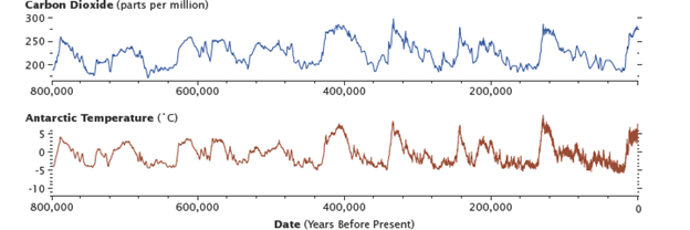
Levels of carbon dioxide in the atmosphere have corresponded closely with temperature over the past 800,000 years. Although the temperature changes were touched off by variations in Earth’s orbit, the increased global temperatures released CO2 into the atmosphere, which in turn warmed the Earth. Antarctic ice-core data show the long-term correlation until about 1900. (Graphs by Robert Simmon, using data from Lüthi et al., 2008, and Jouzel et al., 2007.)
As recorded in CO2 bubbles frozen in glaciers in Antarctica, for the past 800,000 years, the fast and slow carbon cycles have maintained a relatively stable concentration of carbon in all of the carbon reservoirs.
Carbon dioxide, methane, and halocarbons are greenhouse gases that absorb a range of energy, including infrared energy (heat) emitted by the Earth. They then re-emit this energy in all directions, including towards Earth, where it heats the surface. Without these greenhouse gases, Earth would likely not be habitable, but it acts as a dial: with too many, Earth’s temperatures would look more like those of Venus (i.e., 400 degrees Celsius or 750 degrees Farenheit).
But what happens as the amount of carbon dioxide in the atmosphere changes? What will happen to all aspects of the carbon cycle as climate changes? Many researchers are looking into this, including researchers making observations on Earth’s surface, modelers, as well as researchers making observations from satellites.
Carbon measurement Approaches and Accounting Frameworks
According to the State of the Carbon Cycle Report (USGCRP, 2018) Preface (Shrestha et al, 2018), there are three frameworks of observational, analytical, and modeling methods used to estimate carbon stocks and fluxes. These include:
- inventory measurements or a “bottom-up” approach, where total inventory is calculated by gathering data on different stocks of carbon, from biomass, to soil, fresh and saltwater, and areas of exchange among the land, water, and atmosphere (i.e., detailed) and adding all of the quantities together. This includes measurement of carbon emissions from power plants, remote-sensing, field estimates collected spatially and temporally, and more;
- atmospheric measurements or the “top-down” approach, which couples atmospheric gas measurements that have sampled air on the ground, towers, buildings, from balloons, aircrafts, and remote sensors or satellites with tracers and geochemical techniques to broadly examine how gases move in the atmosphere. Top-down estimates have improved significantly in the past 20 years as the types of measurement techniques and diversity of measurements have expanded significantly, such that spatial and temporal resolution across North America has consequently expanded; and
- ecosystem models (as explained in SOCCR2: Appendix D), which use mathematical representations of essential processes in the carbon cycle, such as photosynthesis and respiration, to estimate stocks and fluxes (including information and representation of how environmental parameters impact these processes). Models also are coupled with top-down atmospheric measurements to find the source of greenhouse gas fluxes.
Preface (Shrestha et al. 2018) and Appendix D (Birdsey et al. 2018).
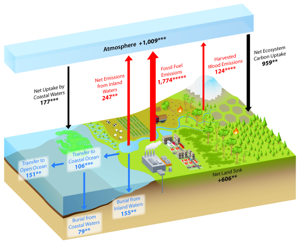
North American Carbon Cycle
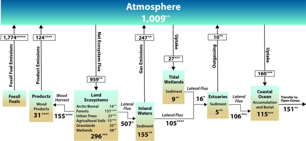
See the Second State of the Carbon Cycle Report.
Since the early 1700s, humans have been releasing carbon into the atmosphere unprecedented amounts of carbon-containing greenhouse gases (GHGs), especially CO2 and CH4. This has largely been from underground, stored carbon that has been sequestered in the lithosphere for tens of millions of years in the form of fossil fuels such as coal, petroleum, natural gas, and more (SOCCR2, Chapter 2; Hayes et. al, 2018). Wildfires and other land disturbances such as land-use change have also been major continental sources of CO2 and CH4.
When considering the whole world, continental sources of carbon are partially offset by natural and managed ecosystem sinks, credence to the “plant a tree” idea. Essentially, in natural and managed ecosystems, plant photosynthesis will convert the atmospheric CO2 into biomass. The terrestrial carbon sink in North America is large, and offsets a large proportion of carbon sources from emissions. Estimates, though uncertain, range from 16% to 52% of carbon source offset by terrestrial ecosystems in North America (King et al., 2015).
Global Carbon Budget
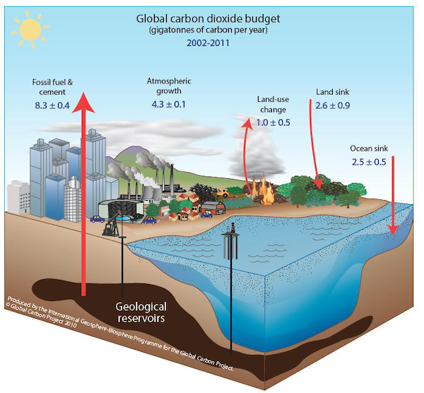
We often talk about carbon in “Gigatons” of carbon, or GtCs.
1 GtC = 1 gigaton of carbon = 109 metric ton carbon or 1 billion tons of carbon. This is equivalent to ~185 million African bush elephants worth of Carbon.
1 PgC = 1 petagram of carbon = 1015 g of carbon
There was CO2 in the atmosphere before humans were around, which is part of why Earth is habitable. But a large percentage of CO2 in the atmosphere has been produced by human beings through the burning of fossil fuels?
Anthropogenic CO2 comes from fossil fuel combustion, changes in land use (e.g., forest clearing), and cement manufacture. Houghton and Hackler have estimated land-use changes from 1850-2000, so it is convenient to use 1850 as our starting point for the following discussion. Atmospheric CO2 concentrations had not changed appreciably over the preceding 850 years (IPCC; The Scientific Basis) so it may be safely assumed that they would not have changed appreciably in the 150 years from 1850 to 2000 in the absence of human intervention.
Atmospheric CO2 concentrations rose from 288 ppmv in 1850 to 422 ppmv in 2025, for an increase of 134 ppmv. In other words, about 30% (134/422) of the additional carbon has remained in the atmosphere, while the remaining 70% has been transferred to the oceans and terrestrial biosphere.
We know this because researchers are constantly working on quantifying the carbon cycle and reducing uncertainty, and thus, carbon budget estimates are a living equation. The latest carbon budget estimates are published in the Global Carbon Project.
Carbon dioxide is not the only greenhouse gas, and examining its potential as a greenhouse gas compared to other ones provides context. Present tropospheric concentrations, global warming potentials (100 year time horizon), and atmospheric lifetimes of CO2, CH4, N2O, CFC-11, CFC-12, CFC-113, CCl4, methyl chloroform, HCFC-22, sulphur hexafluoride, trifluoromethyl sulphur pentafluoride, perfluoroethane, and surface ozone give us insight into how long changes in the atmosphere might last.
View a table presenting data and source for current greenhouse gas concentrations.
We often talk about the carbon cycle from an anthropogenic perspective, but the carbon cycle predates humans and natural sources and sinks are important constituents of the cycle. Some ecosystems are better than others at sequestering carbon. View an illustration of the major world ecosystem complexes ranked by carbon in live vegetation.
Globally, ~50% of annual anthropogenic carbon emissions are offset by marine and terrestrial ecosystem sinks (Le Quéré et al., 2016). Methane emissions and dynamics add additional uncertainty, as there is interaction between CH4 and CO2 in the atmosphere, and, as CH4 source and sink magnitudes are not well constrained and likely underestimated (Bruhwiler et al., 2017; Miller et al., 2013; Turner et al., 2016).
The sum of all national and regional CO2 emission estimates is less than the global totals (i.e., top-down and bottom-up approach estimates don’t match). The difference between the sum of the individual countries (or regions) and the global estimates is generally less than 5%. There are four primary reasons for this.
- global totals include emissions from bunker fuels whereas these are not included in national (or regional) totals. Bunker fuels are fuels used by ships and aircraft in international transportation,
- global totals include estimates for the oxidation of non-fuel hydrocarbon products (e.g., asphalt, lubricants, petroleum waxes, etc.) whereas national totals do not,
- national totals include annual changes in fuel stocks whereas the global total does not, and
- due to statistical differences in the international statistics, the sum of exports from all exporters is not identical to the sum of all imports by all importers.
The history of our focus on the carbon cycle
We talk about climate change and global warming a lot these days, but it first came up in 1896 when S. Arrhenius, published the paper "On the influence of carbonic acid in the air upon the temperature of the ground." The clear increase in atmospheric carbon dioxide was confirmed beginning in the 1930s. Beginning in the late 1950s when highly accurate measurement techniques were developed (the most famous demonstration of this is in C.D. Keeling's record at Mauna Loa, Hawaii). By the 1990s, it was widely accepted (but not unanimously so) that the Earth's surface air temperature had warmed over the past century.
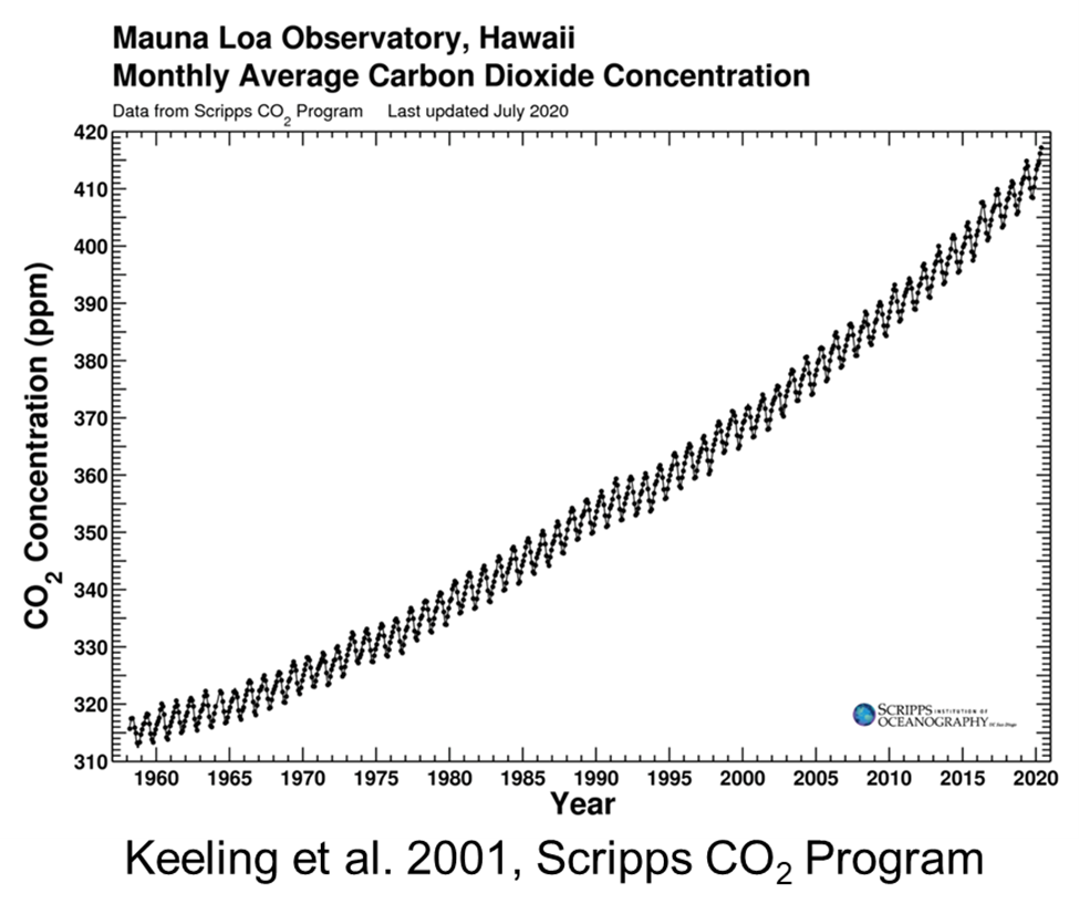
Atmospheric concentration of CO2 as measured at Mauna Loa Observatory in Hawaii, as measured by the Scripps CO2 Program (Keeling et al., 2001) from 1956 to 2020.
It is clear that concentrations of CO2 are increasing, but when we look at a graph of CO2 levels, (for example, Keeling's Mauna Loa data, as seen above), the curve is squiggly, with peaks and troughs every six months. For half of each year, the concentrations increases, and for the other half it decreases. These variations within each year are the result of the annual cycles of photosynthesis and respiration. Photosynthesis, in which plants take up carbon dioxide from the atmosphere and release oxygen, dominates during the warmer part of the year; respiration, by which plants and animals take up oxygen and release carbon dioxide, occurs all the time but dominates during the colder part of the year. Overall, then, carbon dioxide in the atmosphere decreases during the growing season and increases during the rest of the year. Because the seasons in the northern and southern hemispheres are opposite, carbon dioxide in the atmosphere is increasing in the north while decreasing in the south, and vice versa. The magnitude of this cycle is strongest nearer the poles and approaches zero towards the Equator, where it reverses sign. The cycle is more pronounced in the northern hemisphere (which has relatively more land mass and terrestrial vegetation) than in the southern hemisphere (which is more dominated by oceans). The Carbon Cycle Group of the NOAA Climate Monitoring and Diagnostics Laboratory (CMDL), has an excellent 3-dimensional illustration of how atmospheric CO2 varies with time year, season, and latitude.
For further details on the quantitative estimates of sinks, sources, and fluxes of the carbon cycle at present, the latest decadal assessment of the North American Carbon Cyle was published in SOCCR2: the Second State of the Carbon Cycle Report, and the Global Carbon Project has published up-to-date global estimates.
References
Birdsey, R., N. P. Gurwick, K. R. Gurney, G. Shrestha, M. A. Mayes, R. G. Najjar, S. C. Reed, and P. RomeroLankao, 2018: Appendix D. Carbon measurement approaches and accounting frameworks. In Second State of the Carbon Cycle Report (SOCCR2): A Sustained Assessment Report.
Blasing, T. J. (2013). Recent Greenhouse Gas Concentrations. Oak Ridge National Laboratory, Environmental Sciences Division cdiac:doi 10.3334/CDIAC/atg.032. https://data.ess-dive.lbl.gov/view/doi%3A10.3334%2FCDIAC%2FATG.032#ess-dive-af54bad6fc20fe3-20180724T192248766112
Bruhwiler, L. M., Basu, S., Bergamaschi, P., Bousquet, P., Dlugokencky, E., Houweling, S., ... & Weatherhead, E. C. (2017). US CH4 emissions from oil and gas production: Have recent large increases been detected?. Journal of Geophysical Research: Atmospheres, 122(7), 4070-4083.
Hayes, D. J., R. Vargas, S. R. Alin, R. T. Conant, L. R. Hutyra, A. R. Jacobson, W. A. Kurz, S. Liu, A. D. McGuire, B. Poulter, and C. W. Woodall, 2018: Chapter 2: The North American carbon budget. In Second State of the Carbon Cycle Report (SOCCR2): A Sustained Assessment Report [Cavallaro, N., G. Shrestha, R. Birdsey, M. A. Mayes, R. G. Najjar, S. C. Reed, P. Romero-Lankao, and Z. Zhu (eds.)]. U.S. Global Change Research Program, Washington, DC, USA, pp. 71-108, https://doi.org/10.7930/SOCCR2.2018.Ch2.
Houghton, R. A. (1995). Carbon Flux to the Atmosphere from Land-Use Changes: 1850-2005.
cdiac:doi 10.3334/CDIAC/atg.032. https://data.ess-dive.lbl.gov/view/doi%3A10.3334%2FCDIAC%2FLUE.NDP050.2008
IPCC Special Reports on Climate Change. https://www.grida.no/climate/ipcc/
Jouzel, J., Masson-Delmotte, V., Cattani, O., Dreyfus, G., Falourd, S., Hoffmann, G., ... & Wolff, E. W. (2007). Orbital and millennial Antarctic climate variability over the past 800,000 years. Science, 317(5839), 793-796.
Keeling, C. D., Piper, S. C., Bacastow, R. B., Wahlen, M., Whorf, T. P., Heimann, M., & Meijer, H. A. (2001). Exchanges of atmospheric CO2 and 13CO2 with the terrestrial biosphere and oceans from 1978 to 2000. I. Global aspects.
Le Quéré, C., Andrew, R. M., Canadell, J. G., Sitch, S., Korsbakken, J. I., Peters, G. P., ... & Zaehle, S. (2016). Global carbon budget 2016. Earth System Science Data, 8(2), 605-649.
Lüthi, D., Le Floch, M., Bereiter, B., Blunier, T., Barnola, J. M., Siegenthaler, U., ... & Stocker, T. F. (2008). High-resolution carbon dioxide concentration record 650,000–800,000 years before present. Nature, 453(7193), 379-382.
Miller, S. M., Wofsy, S. C., Michalak, A. M., Kort, E. A., Andrews, A. E., Biraud, S. C., ... & Sweeney, C. (2013). Anthropogenic emissions of methane in the United States. Proceedings of the National Academy of Sciences, 110(50), 20018-20022.
NASA (2025). What is the greenhouse effect? National Aeronautics and Space Administration. https://science.nasa.gov/climate-change/faq/what-is-the-greenhouse-effect/
Neftel, A., Friedli, H., Moor, E., Lotscher, H., Oeschger, H., Siegenthaler, U., Stauffer, B. (1997). Historical Carbon Dioxide Record from the Siple Station Ice Core (1734-1983). ess-dive-5207542dddcc7da-20230407T160903163059. doi:10.3334/CDIAC/ATG.010
Olson, J. S., Watts, J. A., Allison, L. J. Major World Ecosystem Complexes Ranked by Carbon in Live Vegetation: A Database (NDP-017) (2001 version of original 1985 data). cdiac:doi 10.3334/CDIAC/lue.ndp017. ess-dive-383d8be5cca5f97-20210429T214148295651
Pro Oxygen (2007). Daily CO2. CO2-Earth. https://www.co2.earth/daily-co2#:~:text=422.78%20ppm&text=This%20table%20presents%20the%20latest,atmospheric%20CO2%20on%20the%20planet
Riebeek, H. (2011, June 16). The Carbon Cycle. NASA Earth Observatory. https://earthobservatory.nasa.gov/features/CarbonCycle
Riebeek, H. (2011, June 16). The Slow Carbon Cycle. NASA Earth Observatory. https://earthobservatory.nasa.gov/features/CarbonCycle/page2.php
Riebeek, H. (2011, June 16). The Fast Carbon Cycle. NASA Earth Observatory. https://earthobservatory.nasa.gov/features/CarbonCycle/page3.php
Riebeek, H. (2011, June 16). Changes in the Carbon Cycle. NASA Earth Observatory. https://earthobservatory.nasa.gov/features/CarbonCycle/page4.php
Shrestha, G., N. Cavallaro, R. Birdsey, M. A. Mayes, R. G. Najjar, S. C. Reed, P. Romero-Lankao, N. P. Gurwick, P. J. Marcotullio, and J. Field, 2018: Preface. In Second State of the Carbon Cycle Report (SOCCR2): A Sustained Assessment Report [Cavallaro, N., G. Shrestha, R. Birdsey, M. A. Mayes, R. G. Najjar, S. C. Reed, P. Romero-Lankao, and Z. Zhu (eds.)]. U.S. Global Change Research Program, Washington, DC, USA, pp. 5-20, https://doi.org/10.7930/SOCCR2.2018.Preface.
Turner, A. J., Jacob, D. J., Benmergui, J., Wofsy, S. C., Maasakkers, J. D., Butz, A., ... & Biraud, S. C. (2016). A large increase in US methane emissions over the past decade inferred from satellite data and surface observations. Geophysical research letters, 43(5), 2218-2224.
Global Carbon Budget (2025). The critical annual update revealing the latest trends in global carbon emission. University of Exeter. https://globalcarbonbudget.org/
USGCRP, 2018: Second State of the Carbon Cycle Report (SOCCR2): A Sustained Assessment Report. [Cavallaro, N., G. Shrestha, R. Birdsey, M. A. Mayes, R. G. Najjar, S. C. Reed, P. Romero-Lankao, and Z. Zhu (eds.)]. U.S. Global Change Research Program, Washington, DC, USA, 878 pp., https://doi.org/10.7930/SOCCR2.2018
